Abstract

Imagine you are responsible for the day-ahead electricity consumption forecast and, from tomorrow, your country is quarantined — a new reality is coming. You are asking yourself: Do I need to change my forecast approach? How do I “explain” to the model that tomorrow is the first day of a new reality? What should I do if the quarantine is prolonged? This is my story: I was responsible for the outcome of the short-term electricity consumption forecast competition. The beginning of the competition coincided with the start of the COVID-19 lockdown in Russia. The forecast service I developed won the competition. In this paper, I draw conclusions and give my answers to the three questions above.

Acknowledgment

The paper is dedicated to my dear friend and mentor Professor Dr. Jury N. Pavlov (1934-2019). I would also like to thank Professor Dr. Anatoly P. Karpenko for his help in editing the manuscript.

I am grateful to AnalyticsHub for the invitation to the forecast project as well as to my colleague Evgenia Maltseva for the daily technical and emotional support and assistance during the competition.

I. Introduction

In Russia, for consumers of the wholesale electricity market, the short-term forecast is performed to bid on the day-ahead market exclusively. A day-ahead bid contains an hourly forecast of the electricity consumption for the so-called hub for the next day. The hub represents a few connected nodes of the power supply system in a certain area. The bid should be submitted to the exchange before 13:30¹ (Figure 1).

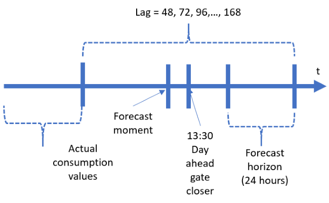
¹Timestamps have hourly resolution and Moscow time zone; power consumption unit is MWh.

Any deviation between actual and day-ahead forecasted consumption will be paid by consumers through the loss-making price of the balancing market, skipping the phase of continuous trading. In the process of continuous trading, market participants make trades in the shared order book. These trades allow participants to reduce the deviation — to balance traded and consumed electricity. Since the continuous trading phase is not developed in Russia, the quality of the day-ahead electricity consumption forecast becomes critical. Further details of the Russian wholesale power market operation can be found in [1].

Under such market conditions, the consumer organizes the day-ahead forecast competition in order to choose the forecast system provider.

The competition rules are as follows: During the agreed period, usually a few months, the competitors receive the latest actual consumption values until 13:00 every working day. The actual values are delayed and the lag value is usually 48, 72, 96… 168 hours (Figure 1). Within 30 minutes, the competitors make the forecast: one day ahead for Monday-Thursday; three days ahead for Friday. The competitors themselves should upload the forecast of the outside temperature, precipitations, and the other variables that impact electricity consumption from the available sources. Thus, the competition rule corresponds to the day-ahead bidding business process of the consumer.

The goal of the competitors is to make the most accurate forecast. Usually, the competitors already have a developed forecast system. Training of the forecast models for a certain hub is done during the preparation phase of the competition. The consumer-organizer provides the historical data of the actual electricity consumption for the previous few years.

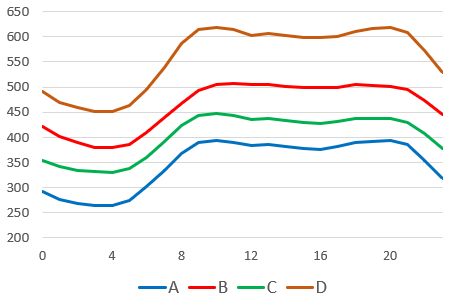
The energy company that organized the competition in question manages the trading activities for a few consumers. Each consumer buys electricity on the wholesale market and sells the purchased electricity to enterprises and the public on the retail market. Sometimes, such companies are called suppliers, but I will continue to refer to them as consumers. An hourly consumption of the four consumers in the competition comprises hundreds of MWh and has a regular daily profile (Figure 2).

During 2019–2020, the energy company held two stages of the forecast competition for four consumers located in different areas of Russia, A, B, C, D:

• Stage 1: 1 September — 30 November 2019
• Stage 2: 1 April — 31May 2020

The start of the second stage of the competition coincided with the beginning of the official lockdown measures in Russia. Unlike developed countries, Russia declared the period from 30 March to 11 May 2020 simply “non-working” and no official quarantine was established. During this period, all activities were stopped except for critical ones. Furthermore, for the period from 12 to 31 May 2020, some activities were either fully or partially permitted. Russia lifted all the lockdown restrictions on 1 June 2020.

I participated in both phases of the competition in collaboration with AnalyticsHub LLC and INFOPRO LLC. My tasks were to develop the forecast model and to win the competition. After the competition was over, the organizer verbally announced the victory of my models on the aggregate of four consumers for both stages ². The full competition results remain closed in accordance with the signed non-disclosure agreement.

² On average, my models scores were the best for both phases. The scoring system resembles that on Kaggle.com.

My most fruitful experience came during the second stage of the competition (the lockdown competition). The main difficulty of the lockdown competition was the parametrization of the “non-working” regime. In other words: how do I explain to the model that a new “non-working” reality is coming which has not occurred in recorded history? In this paper, I give the answer to the question.

The structure of this paper is as follows: the next, section contains a literature review. In the third section, I introduce the forecast service I developed. Finally, in the fourth section, numerical results are discussed.

II. Literature

A. Before the start of the lockdown

Until 31 March 2020, when a first forecast should have been done during the competition, only blogs about how the lockdown impacted electricity consumption were available. With the beginning of the lockdown in Italy, electricity consumption in the third week of March fell by almost 20% compared to the second week [2]. In Spain, the analogous week-to-week reduction was around 6% but here the curvature of the daily profile was noticeable: morning peak hours shifted by 2-3 hours [3].

B. During the lockdown

The COVID-19 pandemic is a unique occasion. Currently, as of February 2020 when I prepared this thesis, there are several studies on the impact of the pandemic on electricity consumption for different countries. In [4], authors explore the issue of the quality of the day-ahead consumption forecast for three regions of the US. The study confirms a noticeable increase of the day-ahead forecast error during the “stay-at-home” regime in two out of three states: New York and Florida. In [5], the authors discuss a significant reduction in electricity consumption of 7-8% compared to the same period in previous years for Poland during the period 1 April — 15 May 2020.

In [6], the authors show that the week-on-week electricity consumption decrease of the first lockdown week in India was the most dramatic at 46%. Moreover, the weekly profile changed significantly: since the beginning of the lockdown, electricity consumption on working days mirrored the weekend in its characteristics. The compact forecast model introduced in [6] has two advantages: it requires a minimum number of actual days for training and it is more efficient than a number of models that the authors refer to as standard (similar day method, multiple regression, autoregression, exponential smoothing). In my opinion, the most vulnerable hypothesis of the authors is the assumption that temperature does not impact the level of electricity consumption during the lockdown. Blogs [2] and [3] and studies [4] and [7] reveal the opposite.

In [7], the authors estimate the day-ahead forecast error made by Terna (Italy’s system operator): during the first days of the lockdown, the average error was roughly four times higher than during normal operations. Week-to-week reduction during the beginning of the quarantine went up to 35% for North Italy. Analogous week-to-week changes for other European countries are introduced in [8].

Finally, it is worth adding that an immaculate review of the electricity consumption forecast studies is introduced in [9]. The research recommendations provided in [9] do not consider the impact of the COVID-19 pandemic.

III. Forecast service

From April to August 2019, at the request of AnalyticsHub, I developed a software service for the day-ahead electricity consumption forecast. The official name is “Analytical system for forecasting consumption in the electric power industry AHUB-Forecasting. Version 2.0,” registration certificate in the territory of Russia No. 2019619309 (the forecast service) ³.

³ The forecast service was developed in Python as Software-as-a-Service. The service is packed into individual docker container and “talks” to data sources and user application with APIs.

Input data for the forecast service are the following:

The daylight profile is a synthetic time series with hourly resolution. Its value equals 0 at night; it linearly increases from 0 to 1 from dawn to zenith; it linearly decreases from 1 to 0 from zenith to sunset.

A. Before the lockdown competition

The forecast service contains a set of mathematical models. The models are applied consequently. The sequence of the model is defined in a specially developed JSON-file. In the same JSON-file, I store hyperparameters of each model. To add a new consumer to the service, you need to:

1. map data sources,
2. set the model sequence and hyperparameters for each model and train the model.

Trained models are stored in the files of a special format using Python.

As a preparation for the forecast competition, the models were trained on an electricity consumption archive length of approximately 50,000 values (6 years). For each consumer, this dataset was divided into training and validation subsets: 4.5 and 1.5 years correspondingly.

Currently, there are five models in the forecast service.

Table 1. Forecast service model list

No.	Model, notation	Type, predictors	Python library
1	Seasonality, S	Multiple linear regression, predictors: trend, sin-like sequences	scikit-learn
2	Temperature, T	Piece-wise linear regression, predictors: temperature, trend, sin-like sequences	scikit-learn
3	Holiday, H	Average value, predictors: reduction of electricity consumption (details below)	Numpy
4	Autoregression, A	Multiple linear regression, predictors: actual consumption lags	scikit-learn
5	Neural network, N	Feed-forward neural network (Keras layer type is Dense), predictors: up to 150 generated from the input data	Keras, TensorFlow

During the development phase and competition 2019, I defined two stacks of the models. Each stack shows the comparable error and comprises diversity which allows the assembling of the stacks to reduce the final forecast error.

Table 2. Model stacks

Stack name	Three regressions, R3	Python library
Model sequence	1) Seasonality 2) Temperature 3) Holiday 4) Autoregression	1) Seasonality 2) Neural network 3) Autoregression
Output notation	LR3	LRNR

During the training, the errors (residuals) of the first model are input data for the next one. For example, the residuals from the seasonality model are input data for the temperature model; in turn, the residuals from the temperature model are input data for the holiday model, and so on. Thus, the process of training the stack is the way to divide electricity consumption values into their components.

During the forecasting, each model in the stack is provided with its predictors. The result of the stack calculation is the sum of the electricity consumption forecast of each model in the stack:

\[ L(t) = S(X_S(t)) + N(X_N(t)) + A(X_A(t)) + \epsilon(t) \]

Here, \[L(t)\] is electricity consumption at time \[t\]; \[X_S(t), X_N(t), X_A(t) \] are predictors vectors for time \[t\]; \[\epsilon(t)\] is forecast error for the same timestamp. In this paper, the errors are evaluated in MAPE values [10].

Each stack is trained individually for each consumer. The lag between available actuals and the end of forecast horizon (Figure 1) deviates from 48 to 168 hours. The lagged predictors (lagged consumption and temperature values) are used in the neural network and autoregression models. In this regard, I train the stack for each lag separately. In other words, for each consumer I train R3 stack for lag 48, then I train the same stack for lag 72, etc. During the forecast process, the forecast service defines the lag value and then calculates the forecast using the stack for the corresponding lag. It is obvious, that the higher the lag value, the higher the forecast error.

As a conclusion from competition 2019, it became clear that the simple assembling of two stacks gives the best accuracy:

\[ \hat{L}(t) = \alpha \cdot \hat{L}_{R3}(t) + (1-\alpha) \cdot \hat{L}_{RNR}(t) \hspace{1cm} (1)\]

where L(t) is electricity consumption forecast for time t. The value of α is set based on the training result.

Holiday model.

In the forecast service, the holidays are set in a separate file that contains the following table (Table 3).

Table 3. Calendar — Holiday features

Dates	Types	Group	Number in group
23.02.2020	2	4	1
24.02.2020	1	4	2
08.03.2020	2	5	1
09.03.2020	1	5	2
30.03.2020	1	5	1
31.03.2020	1	5	2

In Table 3, the holidays are notes as follows:

In the neural network model, the holiday features are used straightforwardly as three predictors. In the holiday model, the reduction in electricity consumption associated with a holiday is calculated as the average hourly deviation for a group of holidays. Remember, the holiday model follows the seasonality and temperature models, so its input values are “cleared” from the corresponding components. For example, for hour 0, the deviation is calculated as follows:

\[ H(X_H(t | h(t) = 0)) = \frac{1}{N} \cdot \sum_{k}^{N} \left ( \epsilon_T^k (t | h(t) = 0) \right ) \]

Here, \[N\] is the number of holidays within a certain group; expression \[\epsilon_T^k (t | h(t) = 0)\] means residuals from the temperature model for timestamps corresponding to hour 0.

From blogs [2] and [3], it is clear that lockdown conditions reduce electricity consumption. As a final step of the lockdown competition preparation, I decided to:

1. define first lockdown days as holiday replacement days for March (Table 3)
2. in equation (1), set \[\alpha = 0.5\] for B-, C-, D-consumers; \[\alpha=0\] for A-consumer.

It did not work out well.

B. Improvements during the lockdown competition

The main feature of the lockdown competition was extremely stressful. As soon as I had actuals for 4-7 days, I discovered that my decisions had been wrong. Step by step, I was able to improve the quality and stabilize the forecast service performance.

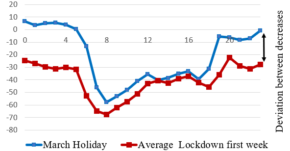
Step 1. R3 stack inefficiency

For the first 4-7 lockdown days, the R3 stack gave significantly poorer results than the RNR stack. A visual analysis of the electricity consumption decreases typical for the March holidays and the consumption decreases due to the lockdown showed their discrepancy (Figure 3). The deviations between these decreases were A — 3%, B — 1%, C — 6%, D — 3% (in percentages from average electricity consumption in the first lockdown week).

I decided to abandon the R3 stack and proceed with the RNR stack only, i.e., set \[\alpha=0\] in the equation (1).

Step 2. Folded neural networks

At the same time, a visual study of the RNR stack results revealed “ripples” in the forecast daily profile (Figure 4). The “ripples” effect is probably the result of a non-balanced train set: there are only 10 days for the March holidays which is not enough for proper network training.

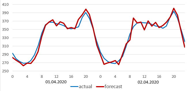
The developed neural network has three layers: the input layer contains from 2,000 to 3,500 neurons (depending on a number of predictors); the hidden layer contains from 48 to 96 neurons (depending on consumer); the output layer contains 24 neurons; loss function is MAE [11].

To eliminate the “ripples” effect, I decided to apply k-fold cross-validation procedure. Python class KFold allows us to split the training dataset into k consecutive folds: one fold is used for testing, the rest for training. As a result, there were k neural networks trained on shuffled subsets. Such cross-validation is widely applied for decision trees like XGBoost, LightGBM, and CatBoost [12]. The final forecast of the cross-validated neural network model is an average of k individual network forecasts.

To define the value of k, I used the following algorithm:

For four consumers, final k = 5.

Step 3. Calendar combination

After one week of the competition, I asked myself: “How would the network stack have performed if it had not known anything about the lockdown?”

The study revealed that the RNR stack trained using the holiday features without any information about the lockdown caught up the performance of the RNR stack trained using holiday features with the lockdown details (RNRLD in Table 3). Both neural network models in the stacks were k-fold trained.

Additionally, I noticed that the forecast error of the weighted combination of RNR and RNRLD was stably lower than both original forecasts. In this respect, I changed the lockdown definition in the holiday features table: lockdown days were allocated to a separate group, the number in the group was a weekday number from 1 to 7 (Table 7). The features of the other holidays remained unchanged.

Table 4. Model stack updated

Stack name	RNR	RNRLD
Model sequence	1) Seasonality 2) Neural network (5-fold, calendar without lockdown definition) 3) Autoregression	1) Seasonality 2) Neural network (5-fold, calendar with lockdown definition) 3) Autoregression

The forecast service was improved to allow two RNR stacks assembling from Table 4 analogously to equation (1). Please, note that the values of the hyperparameters remained unchanged.

For B-consumer, a new forecast service version that included the three steps above was delivered by 10 April 2020. During 13-14 April, the rest of the consumers were moved to the new forecast service. This led to a reduced forecast error.

IV. Numerical results

Remember that competition results are closed in accordance with the signed non-disclosure agreement. Here, I publish only forecast errors obtained with the forecast service.

A. Preparation for the lockdown competition

During preparation for the lockdown competition, I trained two stacks (Table 2). Errors for train (4.5 years) and valid (1.5 years) sets are in Table 5. Autoregression error is the error of the entire stack.

The application of α allows flexibly assembling the stacks. For example, for A-consumer the gain of the RNR (1.53%) is obvious versus R3 (2.09%). Hence, for this consumer, \[\alpha = 0\]; for B-consumer both stack errors are the same, as a result, its \[\alpha = 0.5\].

Table 5. Train and valid MAPE, lag = 48

Stack	Model	MAPE for Training / Validation sets (%)
R3	S	4.57 / 6.55	8.26 / 7.87	4.82 / 8.19	5.68 / 7.56
	T	3.14 / 4.84	4.21 / 4.16	3.87 / 7.63	4.15 / 5.40
	H	2.84 / 4.18	4.09 / 4.01	3.48 / 6.84	3.90 / 4.89
	A	1.99 / 2.09	2.30 / 2.07	2.23 / 2.53	1.97 / 1.97
RNR	S	4.57 / 6.55	8.26 / 7.87	4.82 / 8.19	5.68 / 7.56
	N	1.28 / 1.80	1.82 / 3.40	1.65 / 2.37	1.49 / 1.98
	A	1.27 / 1.53	1.65 / 2.07	1.65 / 2.15	1.47 / 1.67

B. Lockdown competition results

Forecast competition errors are presented in Table 6.

Table 6. Competition monthly MAPE (%)

Month	A	B	C	D
April	2.7	2.2	4.1	3.4
May	2.4	2.5	4.2	3.6

The values in Table 6 show that the error during the competition was 1.5-2 times higher than the valid error (Table 5). This happened partly due to the fact that valid errors are provided for the minimum lag = 48. Meanwhile, during the competition, the lag value deviates in the range 48-168.

In Figure 5, there are three distinguishing periods with high errors. Let’s examine these periods.

1) Initial period

As said in the previous section, until 10 April, the continuous forecast service updates happened. The average error for all four consumers in that period was 3.3%

2) Transient period and central heating switch-off

During 10-14 April, consumers were consequently moved to the new version of the forecast service. During the transient period, the error reduced to 2.8%.

During 15-18 April, in the territories of three of the four consumers, the central water heating switch-off happened. The switching-off process usually continues for 1-3 days and depends on the operation condition of domestic water boilers and combined heat and power plants in the area served by the consumer. This period is usually characterized by increased volatility of consumption: those who get cold, warm up their premises with electric heaters. During the switch-on period, a similar volatility is observed for several days before switching on. The average forecast error in these days increased to 2.9%.

During the final third of April, the forecast error significantly reduced to 1.8%.

3) May holidays

May holidays in Russia consist of two consecutive sets of holidays. In 2020, 1-5 May were holidays (Labor Day), 6-8 of May were lockdown days, 9-11 of May were holidays again (Victory Day). The holiday features for this period are in Table 7. In case of holidays, the forecast horizon is changed from the usual schedule: On 30 April, the forecast was done for six days ahead (1–6 of May, lags 48–168). For 8 May, it was done for four days ahead (9–12 of May, lags up to 120).

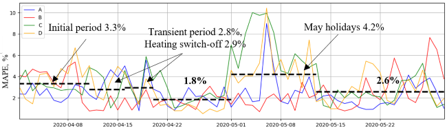
The average error during the May holiday was 4.2%.

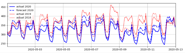
The error for C-consumer was 6.9% — the highest. Figure 6 shows C-consumer’s actual and forecast consumptions. It is noticeable that electricity consumption decrease during May 2020 was the highest in recent years: this decrease in 2020 is two times higher than the corresponding one for 2017-2019. Remember, this decrease excludes seasonal and temperature components.

Table 7. May 2020 Holiday features

Date	Type	Group	Number in group
30.04.2020	1	20	4
01.05.2020	2	7	1
...	...	...	...
05.05.2020	1	7	4
06.05.2020	1	20	3
07.05.2020	1	20	4
08.05.2020	1	20	5
09.05.2020	2	7	5
10.05.2020	1	20	7
11.05.2020	1	7	6
12.05.2020	1	20	2

For the other consumers, the May holidays errors were: A — 3.0%, B — 1.8%, D — 5.1%.

The average error for the rest of May was 2.6%.

V. Conclusion

It is time to answer the three questions from the abstract. Further recommendations relate exclusively to the application of the regression and neural network models for a short-term electricity consumption forecast under a “new reality” condition.

A. Do I need to change my forecasting approach?

If you forecast using regression models and treat holidays in a similar way to that described above, it makes sense to change the approach. Probably it is worth paying attention to the compact forecast model from [6].

If you forecast using neural network models, you do not have to change the approach. However, you should be attentive while parametrizing a new reality.

B. How do I “explain” to the model that tomorrow is the first day of a new reality?

In the first stage, when no actuals are available for the new reality, you may parametrize upcoming days as either the nearest holiday (or replacement day) or the beginning of the lockdown in 2020. It should be expected that the forecast error will be significantly higher for these days.

When actuals for 5-7 days are available, you should update holiday features, put a new reality into a separate group, and retrain the model.

Apply k-fold training, as this will improve forecast quality. During the first month of the new reality, you should retrain the model at least once a week.

C. What should I do if the quarantine is prolonged?

A new reality might consist of stages. For example, the lockdown stages in India [6] and Russia when restrictions were consequently lifted. In that case, it is worth trying to treat each stage as a separate group of holidays.

Continually monitor the behavior of a neural network model trained blindly to a new reality. At some point, errors of two networks might get close. Here, you can

I dare to suggest that even in the case of dramatic electricity consumption changes like in India with its 46% drop, the developed stack RNR^LD would have caught up to the new reality in a few days. The neural network model massively uses electricity consumption lagged variable and has enough capacity to adjust to a new time series behavior quickly.

[1] I. Chuchueva “The Three-Headed Dragon: Electricity, Trading, Analysis”, “Energo-Info” Journal, No. 6, October 2018, pp 32-47

[2] M.-A. Puica “Italian Power Demand Development”, published on 17.03.2020, URL: https://www.linkedin.com/pulse/italian-power-demand-development-mihaela-alexandra-puica/

[3] M.-A. Puica “Spanish Power Demand Development”, published on 18.03.2020, URL: https://www.linkedin.com/pulse/spanish-power-demand-development-mihaela-alexandra-puica/

[4] D. Agdas and P. Barooah, "Impact of the COVID-19 Pandemic on the U.S. Electricity Demand and Supply: An Early View From Data," in IEEE Access, vol. 8, pp. 151523-151534, 2020, doi: 10.1109/ACCESS.2020.3016912.

[5] M. Czosnyka, B. Wnukowska and K. Karbowa, "Electrical energy consumption and the energy market in Poland during the COVID-19 pandemic," 2020 Progress in Applied Electrical Engineering (PAEE), Koscielisko, Poland, 2020, pp. 1-5, doi: 10.1109/PAEE50669.2020.9158771.

[6] S. Lokhande, S. A. Soman and N. Hiremath, "Quick Learn Approach for load forecasting during COVID 19 lockdown," 2020 21st National Power Systems Conference (NPSC), Gandhinagar, India, 2020, pp. 1-6, doi: 10.1109/NPSC49263.2020.9331869.

[7] P. Scarabaggio, M. La Scala, R. Carli, and M. Dotoli, "Analyzing the Effects of COVID-19 Pandemic on the Energy Demand: the Case of Northern Italy," 2020 AEIT International Annual Conference (AEIT), Catania, Italy, 2020, pp. 1-6, doi: 10.23919/AEIT50178.2020.9241136.

[8] Narajewski, Michał & Ziel, Florian. (2020). “Changes in electricity demand pattern in Europe due to COVID-19 shutdowns”.

[9] T. Hong, P. Pinson, Y. Wang, R. Weron, D. Yang and H. Zareipour, "Energy Forecasting: A Review and Outlook," in IEEE Open Access Journal of Power and Energy, vol. 7, pp. 376-388, 2020, doi: 10.1109/OAJPE.2020.3029979.

[10] Mean Absolute Percentage Error. URL: https://en.wikipedia.org/wiki/Mean_absolute_percentage_error

[11] Mean Absolute Error. URL: https://en.wikipedia.org/wiki/Mean_absolute_error

[12] J. Brownlee “XGBoost With Python: Gradient Boosted Trees with XGBoost and scikit-learn,” Machine Learning Mastery, 2016, 115 p.