1. Brief history

The start of the Russian Wholesale Electricity Market in September 2006 made the market price forecast an actual problem. The first scientific attempts to forecast market prices in Russia began in 2009. During the next few years, researchers introduced a number of forecast models which gave more or less reliable results. In this blog, I will introduce the basic idea of the forecast model on the most similar pattern. I developed this model between 2008 and 2013 to address electricity price and consumption forecast problems and it was applied as a core model for the Mathematical Bureau forecast service during 2010-2013.

In 2012, I defended my Philosophy Thesis on the subject The time series forecast model on the most similar pattern at Bauman Moscow State Technical University. The thesis was published in Russian on the website of the Mathematical Bureau and, by the end of 2018, it had received over 65,000 views. The scientific quotation of the thesis has reached 55 according to the Russian Science Index.

The forecast model on the most similar pattern belongs to time series statistical along with ARIMAX, GARCH, ES and others. In the simplest version of the model to calculate forecast values of the target time series, only actuals of this target time series are required. For example, to get price forecast values for the European part of Russia, the so-called European price zone, only price actuals for that price zone are needed. Additionally, the model can take into account external factors which impact the target time series. For example, consumption may be a factor in determining the electricity price. Such factors should be represented as individual time series.

In 2010-2013, based on the model implementation Sergey, a friend of mine and a great software developer, and I attempted to introduce a commercial forecast service for the power market of Russia. The service automatically uploaded price and schedule actuals from the exchange website, forecasted the values and published results on the Mathematical Bureau website. The project had no commercial success due, we suppose, to the immaturity of trading activities in the market. During the project, we improved the model and reached the following error level: day-ahead price forecast errors are in the range 3-8% for the one-day forecast horizon and 6-15% for the week forecast horizon.

The structure of this blog is as follows. In the model framework, the basic idea and algorithm of the forecast model on the most similar pattern are introduced. In the implementation section, the structure of the Mathematical Bureau forecast service and the model implementation features are discussed. The result section is related to forecast error values.

2. Model framework

2.1. Introduction

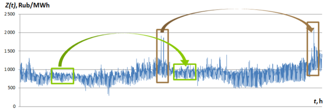
The forecast model on the most similar pattern is based on the idea of the similarity of different pieces of the same time series. In my PhD thesis, the pieces are formally called the patterns and the patterns resemblance — the similarity. In figure 1, the day-ahead price time series and its similar patterns are represented.

Let's denote the time series with \[Z(t)\] and the time series pattern with a start at time step \[t\] and length \[M\] — \[Z^M_t\].

The measure of the similarity of the two patterns with time delay \[k\] is an absolute value of the Pearson linear correlation. Why is that? I've tried a different version of the similarity measure and have found that, for the first iteration, the Pearson linear correlation is the best guess. Specifically, the similarity measure looks like

\[S^M_k = \left | corr(Z^M_t, Z^M_{(t-k)}) \right | \hspace{1cm} (1)\]

Any statistical forecast model is based on an assumption, which is often called a hypothesis. Two assumptions lay in the basement of the model on the most similar pattern.

1. For each pattern \[Z^M_t\] there is the pattern \[Z^M_{t-k}\] which gives a similarity measure close to one.
2. If two patterns \[Z^M_t\] and \[Z^M_{t-k}\] are similar, which means their similarity measure is close to one, their time expansions will be similar as well.

In practice, these assumptions should be verified for each time series individually.

Forecast moment \[T\] is the moment where the actuals end and forecast should be made. Pattern positions and names are shown in figure 2.

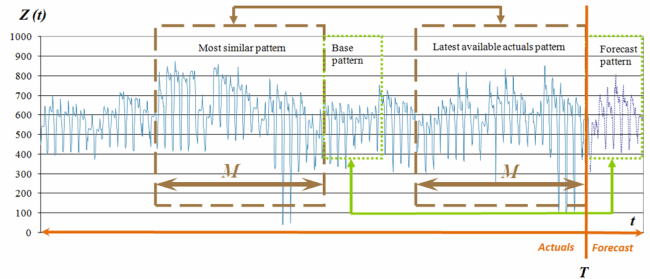
To reiterate our assumptions with given pattern names:

1. We assume that for each latest available actual pattern there is always the most similar pattern with a similarity measure close to one.
2. We assume that the base pattern, a time expansion of the most similar pattern, will have a similarity measure with the further development of the time series (forecast pattern) close to one.

2.2 Algorithm

Let's have a look at the simplest version of the model algorithm. It consists of five steps. An example of the MATLAB code for the model can be found in the blog The time series forecast model on the most similar pattern example in MATLAB.

Step 1. Define the latest available actual pattern.

The latest available actual pattern, denoted \[Z^M_{T-M+1}\], is the most recent actual values.

Step 2. Find the most similar pattern.

To find the most similar pattern all the available patterns of the target time series should be checked using looping through \[k\]. As the looping result, the pattern which gives maximum similarity value is taken. Make sure the similarity value is close to one.

\[ max(S^M_k), \forall k \hspace{1cm} (2)\]

The time delay \[k\], which corresponds to maximum similarity value, denoted with msp. The most similar pattern — \[Z^M_{T-msp}\].

Step 3. Calculate the linear coefficients.

When we talk about the patterns resemblance or similarity, we do not claim that patterns are the same. They are probably not, but they are linear-dependent. Why linear? Because we're checking the exact type of dependence using the Pearson correlation as the similarity measure.

This linear dependency looks like this:

\[Z^M_{T-M+1} = \alpha_1 \cdot Z^M_{T-msp} + \alpha_0 + e \hspace{1cm} (3)\]

In other words, we use simple regression to approximate the latest available actual pattern \[Z^M_{T-M+1}\] with the most similar pattern \[Z^M_{T-msp}\]. Here \[\alpha_1, \alpha_0\] are linear coefficients, \[e\] is an approximation error. The coefficients \[\alpha_1, \alpha_0\] can be calculated a number of ways, I prefer the least mean square method.

Step 4. Define the base pattern.

The base pattern is the time series piece which comes right after the most similar pattern on the time axis (figure 2). Let's denote it \[Z^P_{T-msp+M+1}\]. Here \[P\] is a number of forecast values we're aiming to get, the so-called forecast horizon.

Step 5. Calculate forecast values.

Forecast pattern \[\hat{Z}^P_T\] is calculated using the base pattern and obtained linear coefficients:

\[\hat{Z}^P_T = \alpha_1 \cdot Z^M_{T-msp+M+1} + \alpha_0 \hspace{1cm} (4)\]

Remember that the hat symbol ̂ (hat) is usually used for model results in notations.

Well, that's it, the forecast is done.

As we may see from the algorithm, the only model parameter is \[M\] which represents the pattern's length. Estimation of \[M\] should be done with preliminary looping through possible values, the recommended range \[M \in {2P,…,15P}\]. That looping can be considered as the model calibration.

3. Implementation

3.1 Service

The forecast model on the most similar pattern was coded in MATLAB (2007, 2011b). Furthermore, this implementation was the core of the Mathematical Bureau forecast service (software as a service) for the Wholesale Electricity Market of Russia. The forecast service was launched at the end of 2010 and provided day-ahead price and consumption forecast values automatically. The service software had the following structure (figure 3).

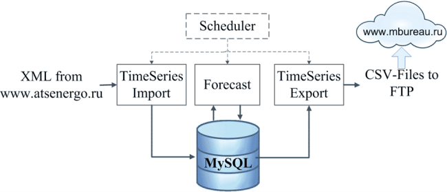
Modules TimeSeries Import, TimeSeries Export and Scheduler were implemented in Java by my friend, Sergey. Module Forecast was implemented in MATLAB by me. We combined these two solutions into one service. The actual and forecast values together with model parameters were stored in a MySQL database. The forecast service didn’t have any User Interface and was controlled by a command prompt.

During 2010-2013 the Mathematical Bureau service forecasted the day-ahead prices for two price zones, five united energy systems and five hub indexes. Thus, the forecast of 12 price time series was carried out daily. The price forecast had two horizons: day-ahead and week ahead, both in hourly resolution.

3.2 Features

The forecast service started to work daily at 17:30 Moscow time. Forecast for the week ahead horizon took place on Wednesday only.

The above-mentioned algorithm looks simple but, in our forecast service, I made a rather complex implementation of the model. For both horizons and each time series, the following procedure was applied.

1. Price forecast #1 was calculated using the target time series (the simplest case, akin to the above-mentioned).
2. A new time series was obtained using the target time series by differencing time step like that \[\tilde{Z}(t) = Z(t) – Z(t-1)\].
3. Price forecast #2 was calculated using a new time series \[ \tilde{Z}(t)\] and the same technique as for forecast #1.
4. The average of two forecasts was calculated. The value could be considered as a consensus-forecast.
5. This consensus-forecast was published on the Mathematical Bureau website.

External factors were not taken into account to improve model performance, because the power market at the time was relatively closed and most of the day-ahead parameters weren't published openly.

4. Results

In 2010, the very first version of the model on the most similar pattern was built. A new version was released in April 2011, and the forecast service was carried out in the way described above. Here, I publish forecast error reports for the period April 2011 to April 2013.

Forecast error is calculated with values MAPE (%), meaning absolute percentage error, and MAE (Rub/MWh), meaning absolute error. Mean error values for the entire 2-year period are represented in table 1.

Day-ahead prices, by areas
	MAE (Rub/MWh)		MAPE (%)
	Day ahead	Week ahead	Day ahead	Week ahead
	24 values	168 values	24 values	168 values
European price zone	52.36	61.58	5.78%	6.98%
Siberian price zone	45.11	59.75	7.03%	9.09%
Ural energy system	53.60	69.00	5.66%	7.31%
Middle Volga energy system	35.00	71.88	3.48%	14.32%
South energy system	66.56	81.29	For these areas, actual prices were sometimes close or equal to 0, which is why the MAPE value goes to infinity.
North-West energy system	72.40	97.46
Centre energy system	56.20	81.50
Centre hub	57.60	80.25
South hub	67.84	84.50
Ural hub	51.68	67.00	5.49%	7.15%
East Siberia hub	46.20	55.29	7.46%	8.90%
West Siberia hub	52.24	70.29	7.81%	10.49%

Brief notes on the table: the Wholesale Power Market of Russia has a nodal pricing system. There are two price zones in Russia — the European and the Siberian. In addition, there are five energy systems, defined by the System Operator and five hubs defined by the market exchange organisation called the Administrator of Trade System. Before 2014 hub prices were used for settling bilateral contracts, currently they are not in use.

The error values were partly published in my PhD thesis in March 2012. A detailed forecast accuracy report by month is available in the file MostSimilarPatterPriceForecast2013.xlsx.