A brief history of the project
At the beginning of April 2019, my former colleague reached out to me. We used to work together on combine and heat power plant optimization projects. He offered me the chance to develop a short-term power consumption forecast system in Python for specific consumers in Russia. After a couple of calls, the details were settled and on April 23rd, on my birthday, I signed my first private contract.
The goal of the work was clearly stated: to develop a short-term power consumption forecast system for distribution companies and end-consumers in the wholesale electricity market of Russia. The system had to provide accurate forecasts for day-ahead bidding. The forecast horizon was equal to 24 hours of the following day.
The primary requirement was that I had to win forecast competition in two distribution companies this year. According to my contract, I can’t name the companies, so I will refer to them as Alpha Distribution and Omega Distribution. Victory in such competitions allows discussing the system deployment for the consumer.
For 3.5 months from the end of April till the beginning of August, I developed what — although you can’t call it a system — was a Python tool for short-term electricity consumption forecast. I was working with a new colleague of mine, Evgenia Maltseva.
The forecast competition in Alpha Distribution took place during August and September 2019 for three consumers. The result of the competition was a draw. Or deuce, as is said in tennis. The forecast errors are in the table below:
| Consumer | Alpha Distribution Forecast |
Our Forecast |
|---|---|---|
| Consumer 1 | 1,9% | 1,9% |
| Consumer 2 | 4,7% | 4,2% |
| Consumer 3 | 2,3% | 2,4% |
You will find the detailed results in the blog Forecast Competition Result in Alpha Distribution. Results for Omega Distribution will be published later as the competition is still ongoing while I’m writing this blog.
Below I make a scratch description of the forecast tool in Python that I’ve been developing these last few months.
The short-term power consumption forecast tool in Python
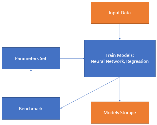
The tool comprises several individually run modules. Each module solves a specific problem. All modules can be divided into two groups: primary and auxiliary. Primary modules train the mathematical models and perform forecasts. Auxiliary modules are related to the extraction-transformation-load (ETL) benchmark and forecast error reporting. In the tool, I implement two types of model: neural network and regression.
The input data for model training and forecasting represents a time series with hourly resolution. We store the time series in individual CSV files. Input data for each consumer to train the model comprises the following values: actual electricity consumption, actual outside temperature, daylight profile, and holiday calendar.
The full competition cycle comprises two stages:
- Train the models.
- Day-by-day forecasting with the trained models during the competition period.
Stage 1. Train the models
Training process
- Upload and evaluate input data, store time series in CSV.
-
Setup initial model predictors and parameters:
- For the neural network model: seasonality as weekday number, week of year number, etc.; weather predictors such as temperature and daylight profile; lags for consumption and temperature; type of network layers; number of neurons; activation function, etc.
- For regression: sin seasonality, weather predictors, trend parameters such as order and type of regression (Linear, Ridge), order and type for auto-regression.
- Split the dataset to train and test parts and train the model.
- Check forecast quality for the test part of the dataset, do a benchmark. Iteratively repeat steps 2, 3, and 4 to achieve the least error.
- Store the model with the best performance.
The first stage is the most time-consuming. Preparing the model for a single consumer may take from a few hours to up to a week of an analyst’s full attention. My colleague trained the neural network models.
The features of the short-term power consumption forecast
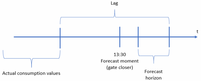
According to the wholesale electricity market of Russia’s rules, consumers may bid for the day-ahead market daily till 13:30 Moscow time, the so-called gate closer. You may explore details of the market functioning in my The Three-Headed Dragon: Electricity, Trading, Analysis paper. Measurement systems collect actual consumption values continuously in different nodes of the power system. Actual hub consumption is an aggregated value, calculated from the measurements. Validation and aggregation require time. Thus, actual values for a specific consumer are available for forecasting with a time delay. For example, each morning only values for two or three days ago are available. If there is any trouble with the measurement system, the delay can be even more — four or five or even more days previous. A lag refers to the number of timesteps between the last available actual value time stamp and the last forecast time stamp. The lag can have values from 24, for one day delay, up to 336, for two weeks delay, in hourly resolution. Lag value is a multiple of 24. To achieve maximum accuracy, we prepared an individual model for each lag. I mean to say that we developed the model for every consumer (hub) for every expected lag value from 24 to 216. In practice, we faced lag equal to 192 and prepared for 216 in case.
Forecast models
As I mentioned above, the developed tool contains two types of model: neural networks and regression. Each model has a specific training module.
1) Neural network
Artificial neural networks are hot nowadays. Except for being a hot topic, neural networks showed high performance at the beginning of 2000 in the consumption forecast problem. I wrote about this in my Ph.D. thesis in 2012.
Today, the most popular neural network framework consists of the triple names: Python and Keras with TensorFlow backend. We followed the fashion in this case and applied exactly that combination in our consumption forecast tool. We constructed a network with Dense layers; a number of predictors varying from 100 to 170 and a number of optimized network parameters varying from 70,000 to 120,000.
Our experiments showed that neural network residuals (in other terms error) are not white noise. We applied the auto-regression model to reduce it.
2) Regression
For a lot of problems in the areas of image recognition or text treatment, regression models are not applicable. But for the short-term consumption forecast problem, it still works well and successfully challenges neural network models.
My regression model is a sequence of three compact regression models:
- Seasonality model. Model input is actual consumption values; model extracts evident yearly and hourly seasonality.
- Temperature model. Residuals from the seasonality model are used as an input for the temperature model. Nowadays, implementation is done as piecewise linear regression or gradient boosting.
- Auto-regression. Residuals from the temperature models are put into the auto-regressive model. The order of auto-regression can reach a few hundred.
Applied technology: Python together with Scikit-learn for regressions and XGBoost package for gradient boosting.
For each consumer, we prepared individual neural network models for each lag value and individual regression models for each lag value. Each model was stored in a separate pickle file. Altogether, the model bunch for each consumer contained nine regression models for lags from 24 to 216 and nine neural network models for the same lag values.
Stage 2. Daily forecasting
Before the start of the competition, a bunch of models was prepared for each consumer from the competition list. Tremendous job!
When the competition started, we made a daily forecast using a separate forecasting module developed for that purpose. This module does the following:
- Upload updated data for actual values that come from the measurement system.
- Define lag value.
- Upload the neural network and regression models for the lag from our model storage.
- Calculate forecast using the regression model.
- Calculate forecast using the neural network model.
- Calculate the average of two independent forecasts; we call this average consensus forecast.
- Make plot.
- Calculate error values for a certain period backward.
- Choose the model to apply on that exact day in Python console line.
- Write forecast values for a required date in a CSV file.
ETL functions, like grab actual temperature values or forecast temperature values, were implemented in auxiliary Python modules. These modules parse CSV or XLS files from local folders or the Internet using API and store the values in local data storage.
Additionally, while the competition was going, we prepared a couple of internal reports for error monitoring and assessment of the choice of the model by an analyst. These functions were implemented as an auxiliary module as well.
Further development
The next obvious step is the development of a short-term power consumption forecast system based on the current tool. The system is planned to be implemented as Software as a Service and will allow flexible integration with any external data source. We plan neither development of comprehensive ETL functionality nor graphical user interface. For our SaaS system data, the source will be an external DBMS. Mathematical algorithm development will remain in the Python environment, like PyCharm and Jupyter Notebook. Part of the new functionality planned will be implemented in Python, the rest in Java.
As further mathematical development, I see adding gradient boosting as a separate forecast model alongside regression and neural networks. Maybe I’ll continue to research developing a residual model based on Empirical Mode Decomposition which extracts low-frequency components of the error (residual) values. Some of the work described here was done in July, but I haven’t developed an efficient solution so far. And finally, I’ve been thinking of including my forecast model on the most similar pattern as a separate module. Implementation of the model in MATLAB showed highly accurate results back in 2010-2012. Maybe it’s time to bring the model back to life in Python.